Zeta Potential from Molecular Dynamics Simulations

g_mu is a utility written in FORTRAN designed to analyze trajectories from nonequilibrium molecular dynamics (NEMD) simulations. This tool was developed within the project aimed to investigate electrokinetic phenomena at solid/liquid interfaces. g_mu allows to calculate the temperature components, streaming velocities of water and ions, and streaming mobilities (if the electric field and charge scaling factor are provided). The latter can be then converted to the zeta potential. For the analysis, a text version (Gromacs .gro format) of a trajectory file (generalization for reading .xtc files is in development) is required. Additionally, g_mu can read a custom format of LAMMPS outputs.

Examples of g_mu outputs are given below. The tested system was the most negatively charged (−0.12 C/m²) quartz (101) surface in 0.33 M NaCl solution with an applied electric field of 0.07 V/nm. NEMD simulations were carried out either in Gromacs with source code modifications, which allow to run simulations with thermostatting only selected velocity components (particularly, only y and z), or in LAMMPS, where this feature is implemented by default. For more details, refer to the publication number three in the list above.

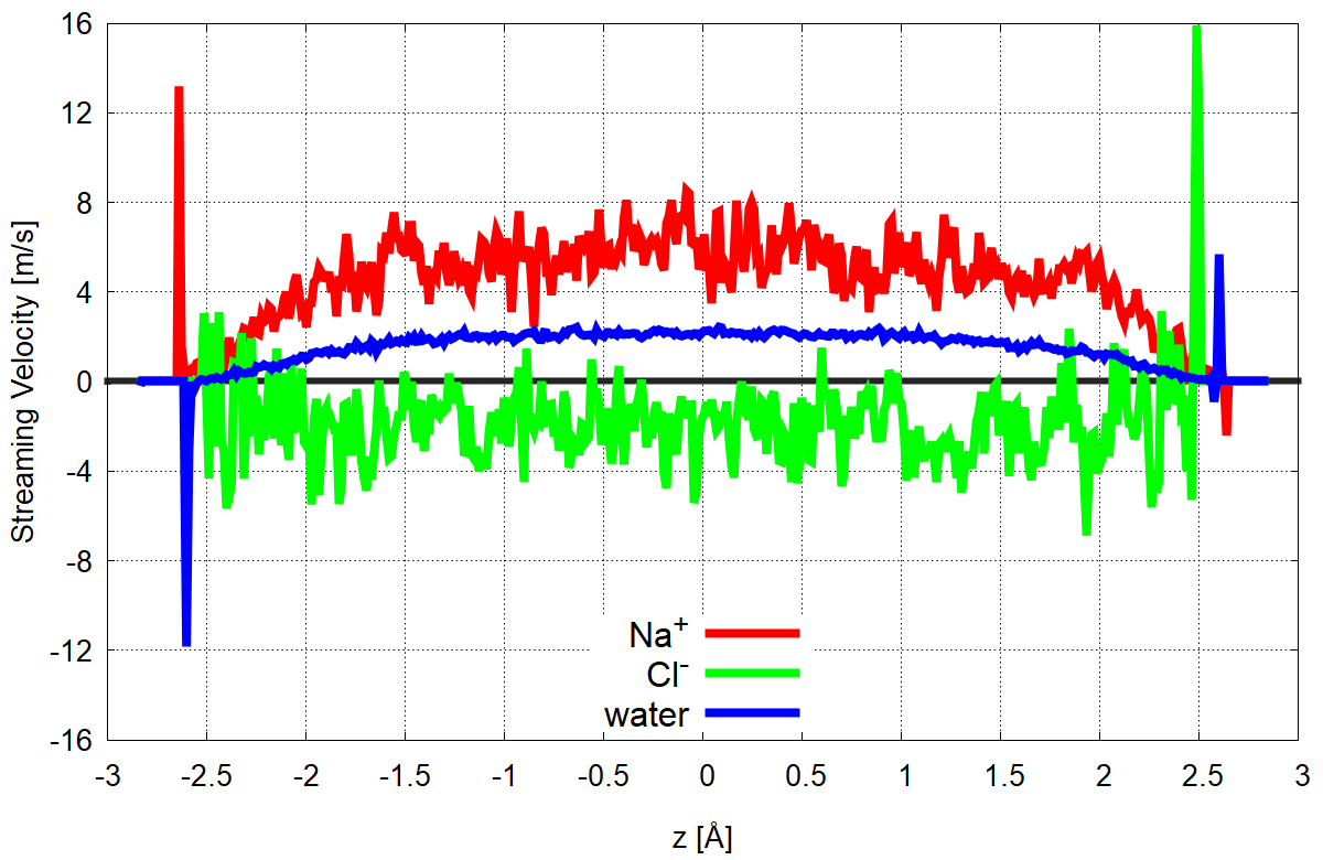
Figure 1. Streaming velocity of water and ions as a function of z-coordinate. Zero is normalized to the center of the simulation box.

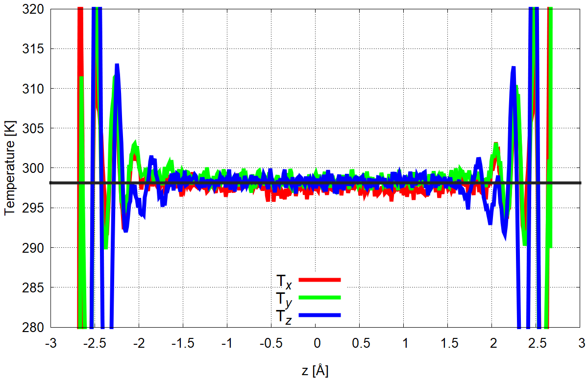
Figure 2. Temperature as a function of z-coordinate calculated separately from all velocity components of water and ions. Zero is normalized to the center of the simulation box.

All input switches and their description can be found when typing g_mu -h.

The most important are following:

• -f − input trajectory file.

• -group − groups of atoms to analyze. Should be specified as the atomic name in the trajectory, i.e. "OW" (water oxygens), "NA" (sodium ions), etc. For instance, -group NA CL OW HW.

• -lmp − switch to LAMMPS.

Files:

• g_mu − linux executable

• gromacs.tar.gz − example input file in .gro Gromacs format

• lammps.tar.gz − example input file in custom LAMMPS format

NOTE! The last two are small files for testing purposes (only 100 saved configurations), while all the published data and representative figures above were obtained from full-fledged, much larger trajectories.

How to deal with these example files?

To analyze Gromacs .gro file, execute following:
g_mu -f gromacs.gro -group NA CL OW HW -left 22.165 -right 27.835 -sl 450 -E-x 0.07 -scale 0.75, where -left and -right define the position of solid walls (surfaces), between which the solution is, -sl is number of bins (slides), -E-x is the amplitude of the applied electric field, -scale is a charge scaling factor (see the manuscript for more details).

To analyze LAMMPS .fake-gro file, the executing command is:
g_mu -f lammps.fake-gro -lmp -group NA CL OW HW -left 1.165 -right 6.835 -E-x 0.07 -scale 0.75 -sl 450, i.e. only a switch -lmp was added and the walls were shifted in our simulations compared to Gromacs.

In both cases, output should be like this:

opening gromacs.gro
Successfully opened gromacs.gro
Analyzing VELOCITIES
Estimated # of frames 101
-----------------------------------
Group Name Atoms Mass
1 NA 48 22.98977
2 CL 16 35.45300
3 OW 3745 15.99940
4 HW 7490 1.00800
5 COM 3745 18.01540
Processing Elapsed Remaining
frame time time
hh:mm:ss hh:mm:ss
100 00:00:03 00:00:00
All molecules were compact in XYZ
Time difference between frames [ps]: 1.00000, number of frames: 101
Distances OW-HW [A] min.: 0.985, max.: 1.014
Maximum dX of any atom: 0.57 nm, i.e. 10% of Lx= 5.50000
Maximum dZ of any atom: 0.62 nm, i.e. 9% of right-left= 6.67000 bins 43
Program ran 3.947266 s

The list of generated files:

dens.dat
dens_norm.dat
ekin.dat
mu.dat
stat.dat
temp_CL.dat
temp_COM.dat
temp.dat
temp_HW.dat
temp_NA.dat
temp_OW.dat
vel.dat
walls.dat